Calibration
Quick start guide
A series of sample images can be downloaded from here.
1. Camera calibration
The first step in any analysis is to perform a camera calibration.
Select + in the Calibration Library.

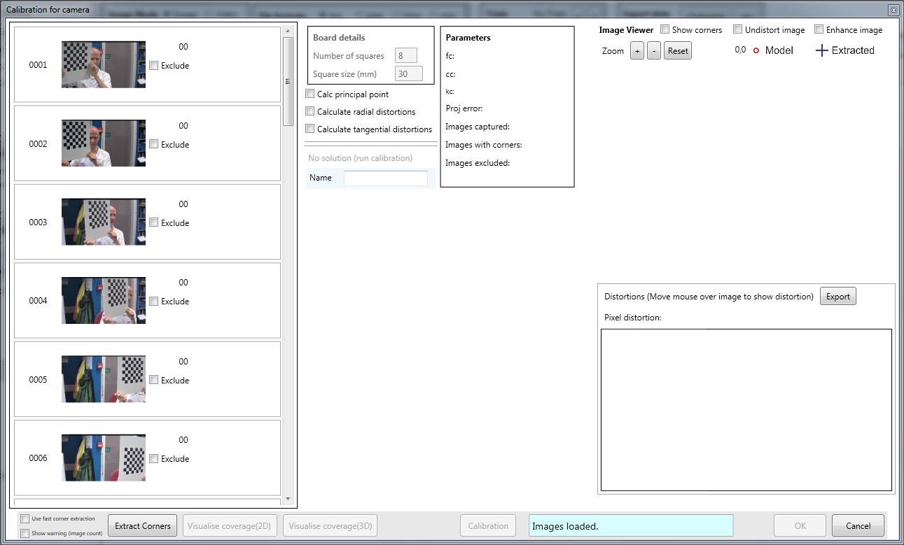
Enter the relevant board details for your specific analysis. The values for the sample images are given in the above screenshot.
Click Proceed to continue.
Extract corners
A camera calibration window will appear (as shown above). The calibration images are shown in the left hand side of the window. Click 'Extract corners' and wait for the operation to complete (this may take over a minute if you have got a large number of images). If a very large number of images have been used, select the 'Use fast corner extraction' option. If the checkerboard cannot be found, the image will be automatically excluded.
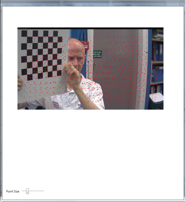
Once the corner extraction has completed, click on 'Visualise Coverage (2D)' to show an image of the calibration with all extracted corners superimposed on it. The size of each point can be adjusted, as shown in the image below.
Calibration step
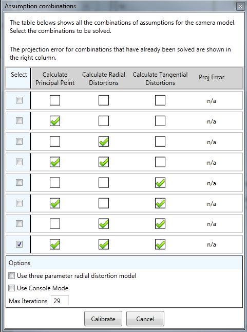
- Click on the 'Calibration' and this loads a page which allows to define which combinations of parameters are solved for the model(s).
- Initially, only select the last combination of model assumptions, as shown above.
- If you are interested in following the progress of the optimisation technique (the solver for the model), select the 'Use console mode' function.
- Set the maximum number of iterations allowed (before the solver will terminate). If the optimisation achieves the defult tolerance it will terminate before this maximum number of iterations is reached. Solutions can be continued, so it is advisable to limit the number of iterations as appropriate.
When the optimisation technique has completed, the calibration parameters are shown in main window. If multiple combinations have been calculated, use the tick boxes to select the required combination (to be viewed).
Calibration review

The calibration output can be reviewed in a number of ways:
-
The proj. error value is the root mean square error (RMSE) of the
reprojection. This is calculated from the distances between the
extracted checkerboard points and the projected points (calculated from
the board extrinsic parameters and the converged solution for the camera
model). This quantifies the accuracy of the model.
-
The individual errors for each reconstruction point are shown in
the chart. Furthermore, the number alongside each calibration
image is the RMSE pixel error for each checkerboard. If any
image has a pixel error which is considerably larger (as a
guide, double the overall projection error), you should consider
excluding that image. Alternatively, if any points in the chart
are show considerably larger errors than the RMSE, then the
image associated with this point should be excluded. (Hover
over the point and it will reveal which image it belongs to.)
- Click Visualise coverage (3D) to display a 3D visualisation of the checkerboard images . The user can rotate the view as appropriate. From this screen, the user can export the board normal vectors to .csv. It is important that the board has been rotated through a wide range of angles (Zhang 1999) and inspection of the board normal vectors can be used to qualititively assess whether the board has been rotated sufficiently. This is described further here.
-
When an image is clicked it appears in the Image Viewer. This
shows the extracted corners, the modelled corners and the search
area used to determine location of the extracted corners. A
zoom rectangle can be used to zoom in. Clicking 'Undistort
image' will apply the lens distortion correction model to
the image.
-
The image in the bottom-right of the screen should show a circle
(geometrical centre of the image) and a crosshair (calculated
principal point of the camera). If the lens is correctly aligned to
the sensor then the
two points should be very close. If they are not close, the user
must decide if they solution is feasible. (i.e. could the lens
be physically misaligned by the same magnitude as calculated by the
model). If this is unlikely, it is advisable to Fix principal point
and run the
calibration again.
- Furthermore, move the mouse over the image in the bottom-right of the screen and this will display the calculated radial and tangential distortion (in pixels) at any point in the image. If either of these distortions are negligble, it is worth rerunning the calibration with the relevant distortion parameter removed. It is generally advisable to ignore tangential distortions in consumer level cameras because the radial component is the dominant distortion. Furthermore, including it where it is not needed can lead to numerical instability in the model (Zhang 1999). It is analogous to fitting a high order trend line to a scatter plot that should actually be represented by a linear trendline.
Calibrations can be rerun, and if the 'console mode' is NOT used, the solver will run in parallel or mult-CPU machines. The general aim in any calibration is to obtain the lowest projection error (RMSE) whilst using the simplest and most relevant model.
When you are happy with the calibration, click OK to save the calibration. Make sure a name is assigned and the desired combination of model parameters is selected when OK is pressed.
For a description of the camera parameters have a look at the Jean-Yves Bouguet's camera calibration site.
2. Origin definition
 This stage can be skipped if you do not want to define a local
coordinate system for the work. In this section, the user needs to
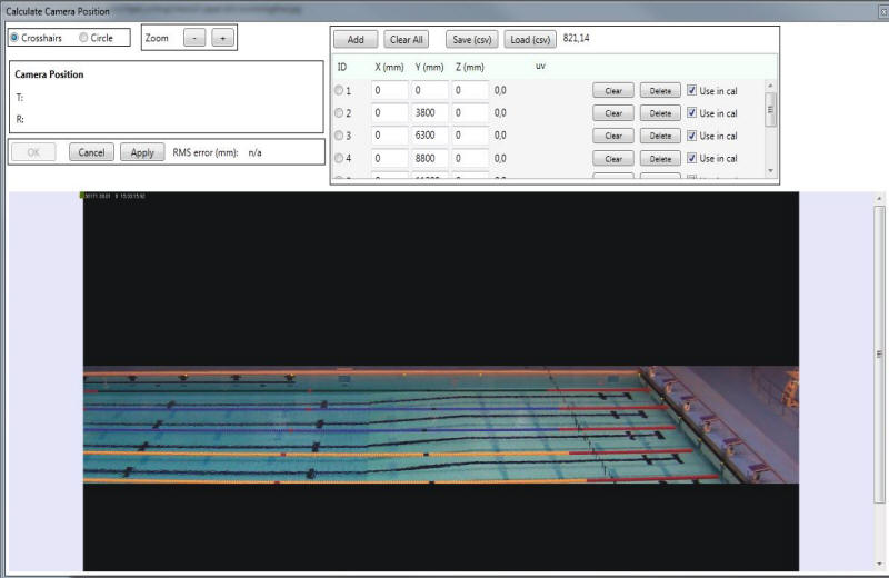
specify atleast four (known) points. In this example, these
points are marked as yellow crosses in the sample image.
(There is an image in the DemoImages of a swimming pool that can be
used to define the origin for the example called OriginDefinition.jpg)
This stage can be skipped if you do not want to define a local
coordinate system for the work. In this section, the user needs to
specify atleast four (known) points. In this example, these
points are marked as yellow crosses in the sample image.
(There is an image in the DemoImages of a swimming pool that can be
used to define the origin for the example called OriginDefinition.jpg)
- Select the appropriate calibration from the library.
- Select the appropriate Image Mode and then
either browse (or drag/drop) and folder or file depending on which
is appropriate. If using images, select the first folder that
contains the image that will be used to define the plane (and
origin). If using a video, simply select the video.
- When the correct image is shown in the main window, select 'Define'
from Origin Definition. In the launched window, either add the
correct number of control points or just load the PoolPoints.csv
file from the downloaded zip file.
-
In the example, the x-axis runs along the lanes and the
y-axis runs along the wall with the starting blocks
-
Click the radio button next to each marker and then click on the
appropriate marker in the image. Once all markers have been clicked
(and all 'Use in cal' checkboxes are ticked) click
on 'Apply'. Check2D should calculate the extrinsic
parameters of the camera (Rotation R and Translation T).
The RMS error in this example should be less than 40 mm.
-
The origin 'triad' will be shown briefly, and in this example, it
should be at the top-right hand corner.
- Click OK to save the calibration. The reconstruction results (including R and T) can be exported from the Export function in the Origin Definition panel.
This completes the specification of the origin system, and any coordinate obtained using this calibration will be referenced to this origin. The calibration file will be saved in the '..\MyDocuments\Check2D\Calibration' folder, and listed in the Calibration Library in Check2D. The uniqueID is used to identify the calibration and is the same as the filename.
Calibrations can be exported/imported so that they can be used on other computers.
References
Zhang, Z., 1999. Flexible Camera Calibration by Viewing a Plane from Unknown Orientations. In: International Conference on Computer Vision, Corfu, Greece, 666-673.